Cube Interpolation and Regridding
Iris provides powerful cube-aware interpolation and regridding functionality, exposed through Iris cube methods. This functionality is provided by building upon existing interpolation schemes implemented by SciPy.
In Iris we refer to the available types of interpolation and regridding as schemes. The following are the interpolation schemes that are currently available in Iris:
linear interpolation (
iris.analysis.Linear), andnearest-neighbour interpolation (
iris.analysis.Nearest).
The following are the regridding schemes that are currently available in Iris:
linear regridding (
iris.analysis.Linear),nearest-neighbour regridding (
iris.analysis.Nearest), andarea-weighted regridding (
iris.analysis.AreaWeighted, first-order conservative).
The linear, nearest-neighbor, and area-weighted regridding schemes support lazy regridding, i.e. if the source cube has lazy data, the resulting cube will also have lazy data. See Real and Lazy Data for an introduction to lazy data.
Interpolation
Interpolating a cube is achieved with the interpolate()
method. This method expects two arguments:
the sample points to interpolate, and
the second argument being the interpolation scheme to use.
The result is a new cube, interpolated at the sample points.
Sample points must be defined as an iterable of (coord, value(s)) pairs.
The coord argument can be either a coordinate name or coordinate instance.
The specified coordinate must exist on the cube being interpolated! For example:
coordinate names and scalar sample points:
[('latitude', 51.48), ('longitude', 0)],a coordinate instance and a scalar sample point:
[(cube.coord('latitude'), 51.48)], anda coordinate name and a NumPy array of sample points:
[('longitude', np.linspace(-11, 2, 14))]
are all examples of valid sample points.
The values for coordinates that correspond to date/times can be supplied as
datetime.datetime or cftime.datetime instances,
e.g. [('time', datetime.datetime(2009, 11, 19, 10, 30))]).
Let’s take the air temperature cube we’ve seen previously:
>>> air_temp = iris.load_cube(iris.sample_data_path('air_temp.pp'))
>>> print(air_temp)
air_temperature / (K)               (latitude: 73; longitude: 96)
     Dimension coordinates:
          latitude                           x              -
          longitude                          -              x
     Scalar coordinates:
          forecast_period: 6477 hours, bound=(-28083.0, 6477.0) hours
          forecast_reference_time: 1998-03-01 03:00:00
          pressure: 1000.0 hPa
          time: 1998-12-01 00:00:00, bound=(1994-12-01 00:00:00, 1998-12-01 00:00:00)
     Attributes:
          STASH: m01s16i203
          source: Data from Met Office Unified Model
     Cell methods:
          mean within years: time
          mean over years: time
We can interpolate specific values from the coordinates of the cube:
>>> sample_points = [('latitude', 51.48), ('longitude', 0)]
>>> print(air_temp.interpolate(sample_points, iris.analysis.Linear()))
air_temperature / (K)               (scalar cube)
     Scalar coordinates:
          forecast_period: 6477 hours, bound=(-28083.0, 6477.0) hours
          forecast_reference_time: 1998-03-01 03:00:00
          latitude: 51.48 degrees
          longitude: 0 degrees
          pressure: 1000.0 hPa
          time: 1998-12-01 00:00:00, bound=(1994-12-01 00:00:00, 1998-12-01 00:00:00)
     Attributes:
          STASH: m01s16i203
          source: Data from Met Office Unified Model
     Cell methods:
          mean within years: time
          mean over years: time
As we can see, the resulting cube is scalar and has longitude and latitude coordinates with the values defined in our sample points.
It isn’t necessary to specify sample points for every dimension, only those that you wish to interpolate over:
>>> result = air_temp.interpolate([('longitude', 0)], iris.analysis.Linear())
>>> print('Original: ' + air_temp.summary(shorten=True))
Original: air_temperature / (K)               (latitude: 73; longitude: 96)
>>> print('Interpolated: ' + result.summary(shorten=True))
Interpolated: air_temperature / (K)               (latitude: 73)
The sample points for a coordinate can be an array of values. When multiple coordinates are provided with arrays instead of scalar sample points, the coordinates on the resulting cube will be orthogonal:
>>> sample_points = [('longitude', np.linspace(-11, 2, 14)),
...                  ('latitude',  np.linspace(48, 60, 13))]
>>> result = air_temp.interpolate(sample_points, iris.analysis.Linear())
>>> print(result.summary(shorten=True))
air_temperature / (K)               (latitude: 13; longitude: 14)
Interpolating Non-Horizontal Coordinates
Interpolation in Iris is not limited to horizontal-spatial coordinates - any coordinate satisfying the prerequisites of the chosen scheme may be interpolated over.
For instance, the iris.analysis.Linear scheme requires 1D numeric,
monotonic, coordinates. Supposing we have a single column cube such as
the one defined below:
>>> cube = iris.load_cube(iris.sample_data_path('hybrid_height.nc'), 'air_potential_temperature')
>>> column = cube[:, 0, 0]
>>> print(column.summary(shorten=True))
air_potential_temperature / (K)     (model_level_number: 15)
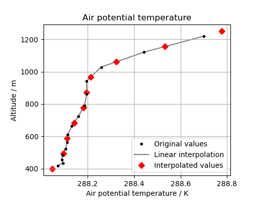
This cube has a “hybrid-height” vertical coordinate system, meaning that the vertical coordinate is unevenly spaced in altitude:
>>> print(column.coord('altitude').points)
[ 418.69836  434.5705   456.7928   485.3665   520.2933   561.5752
  609.2145   663.2141   723.57697  790.30664  863.4072   942.8823
 1028.737   1120.9764  1219.6051 ]
We could regularise the vertical coordinate by defining 10 equally spaced altitude sample points between 400 and 1250 and interpolating our vertical coordinate onto these sample points:
>>> sample_points = [('altitude', np.linspace(400, 1250, 10))]
>>> new_column = column.interpolate(sample_points, iris.analysis.Linear())
>>> print(new_column.summary(shorten=True))
air_potential_temperature / (K)     (model_level_number: 10)
Let’s look at the original data, the interpolation line and the new data in a plot. This will help us to see what is going on:
(Source code, png)

The red diamonds on the extremes of the altitude values show that we have extrapolated data beyond the range of the original data. In some cases this is desirable but in other cases it is not. For example, this column defines a surface altitude value of 414m, so extrapolating an “air potential temperature” at 400m makes little physical sense in this case.
We can control the extrapolation mode when defining the interpolation scheme. Controlling the extrapolation mode allows us to avoid situations like the above where extrapolating values makes little physical sense.
The extrapolation mode is controlled by the extrapolation_mode keyword.
For the available interpolation schemes available in Iris, the extrapolation_mode
keyword must be one of:
extrapolate– the extrapolation points will be calculated by extending the gradient of the closest two points,
error– a ValueError exception will be raised, notifying an attempt to extrapolate,
nan– the extrapolation points will be be set to NaN,
mask– the extrapolation points will always be masked, even if the source data is not a MaskedArray, or
nanmask– if the source data is a MaskedArray the extrapolation points will be masked. Otherwise they will be set to NaN.
Using an extrapolation mode is achieved by constructing an interpolation scheme
with the extrapolation mode keyword set as required. The constructed scheme
is then passed to the interpolate() method.
For example, to mask values that lie beyond the range of the original data:
>>> scheme = iris.analysis.Linear(extrapolation_mode='mask')
>>> new_column = column.interpolate(sample_points, scheme)
>>> print(new_column.coord('altitude').points)
[-- 494.44451904296875 588.888916015625 683.333251953125 777.77783203125
 872.2222290039062 966.666748046875 1061.111083984375 1155.555419921875 --]
Caching an Interpolator
If you need to interpolate a cube on multiple sets of sample points you can ‘cache’ an interpolator to be used for each of these interpolations. This can shorten the execution time of your code as the most computationally intensive part of an interpolation is setting up the interpolator.
To cache an interpolator you must set up an interpolator scheme and call the scheme’s interpolator method. The interpolator method takes as arguments:
a cube to be interpolated, and
an iterable of coordinate names or coordinate instances of the coordinates that are to be interpolated over.
For example:
>>> air_temp = iris.load_cube(iris.sample_data_path('air_temp.pp'))
>>> interpolator = iris.analysis.Nearest().interpolator(air_temp, ['latitude', 'longitude'])
When this cached interpolator is called you must pass it an iterable of sample points that have the same form as the iterable of coordinates passed to the constructor. So, to use the cached interpolator defined above:
>>> latitudes = np.linspace(48, 60, 13)
>>> longitudes = np.linspace(-11, 2, 14)
>>> for lat, lon in zip(latitudes, longitudes):
...     result = interpolator([lat, lon])
In each case result will be a cube interpolated from the air_temp cube we
passed to interpolator.
Note that you must specify the required extrapolation mode when setting up the cached interpolator. For example:
>>> interpolator = iris.analysis.Nearest(extrapolation_mode='nan').interpolator(cube, coords)
Regridding
Regridding is conceptually a very similar process to interpolation in Iris. The primary difference is that interpolation is based on sample points, while regridding is based on the horizontal grid of another cube.
Regridding a cube is achieved with the cube.regrid() method.
This method expects two arguments:
another cube that defines the target grid onto which the cube should be regridded, and
the regridding scheme to use.
Note
Regridding is a common operation needed to allow comparisons of data on different grids. The powerful mapping functionality provided by cartopy, however, means that regridding is often not necessary if performed just for visualisation purposes.
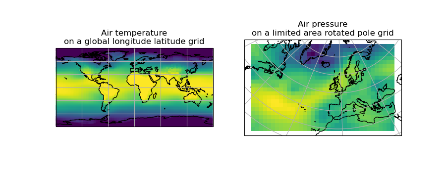
Let’s load two cubes that have different grids and coordinate systems:
>>> global_air_temp = iris.load_cube(iris.sample_data_path('air_temp.pp'))
>>> rotated_psl = iris.load_cube(iris.sample_data_path('rotated_pole.nc'))
We can visually confirm that they are on different grids by plotting the two cubes:
(Source code, png)
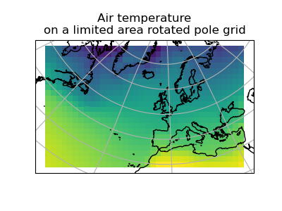
Let’s regrid the global_air_temp cube onto a rotated pole grid
using a linear regridding scheme. To achieve this we pass the rotated_psl
cube to the regridder to supply the target grid to regrid the global_air_temp
cube onto:
>>> rotated_air_temp = global_air_temp.regrid(rotated_psl, iris.analysis.Linear())
(Source code, png)
We could regrid the pressure values onto the global grid, but this will involve some form of extrapolation. As with interpolation, we can control the extrapolation mode when defining the regridding scheme.
For the available regridding schemes in Iris, the extrapolation_mode keyword
must be one of:
extrapolate–
nan– the extrapolation points will be be set to NaN.
error– a ValueError exception will be raised, notifying an attempt to extrapolate.
mask– the extrapolation points will always be masked, even if the source data is not a MaskedArray.
nanmask– if the source data is a MaskedArray the extrapolation points will be masked. Otherwise they will be set to NaN.
The rotated_psl cube is defined on a limited area rotated pole grid. If we regridded
the rotated_psl cube onto the global grid as defined by the global_air_temp cube
any linearly extrapolated values would quickly become dominant and highly inaccurate.
We can control this behaviour by defining the extrapolation_mode in the constructor
of the regridding scheme to mask values that lie outside of the domain of the rotated
pole grid:
>>> scheme = iris.analysis.Linear(extrapolation_mode='mask')
>>> global_psl = rotated_psl.regrid(global_air_temp, scheme)
(Source code, png)
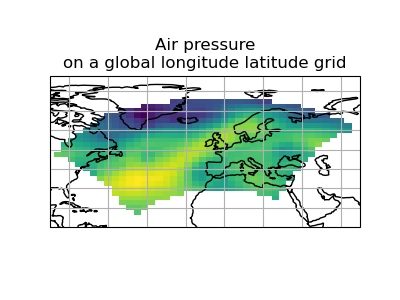
Notice that although we can still see the approximate shape of the rotated pole grid, the cells have now become rectangular in a plate carrée (equirectangular) projection. The spatial grid of the resulting cube is really global, with a large proportion of the data being masked.
Area-Weighted Regridding
It is often the case that a point-based regridding scheme (such as
iris.analysis.Linear or iris.analysis.Nearest) is not
appropriate when you need to conserve quantities when regridding. The
iris.analysis.AreaWeighted scheme is less general than
Linear or Nearest, but is a
conservative regridding scheme, meaning that the area-weighted total is
approximately preserved across grids.
With the AreaWeighted regridding scheme, each target grid-box’s
data is computed as a weighted mean of all grid-boxes from the source grid. The weighting
for any given target grid-box is the area of the intersection with each of the
source grid-boxes. This scheme performs well when regridding from a high
resolution source grid to a lower resolution target grid, since all source data
points will be accounted for in the target grid.
Let’s demonstrate this with the global air temperature cube we saw previously, along with a limited area cube containing total concentration of volcanic ash:
>>> global_air_temp = iris.load_cube(iris.sample_data_path('air_temp.pp'))
>>> print(global_air_temp.summary(shorten=True))
air_temperature / (K)               (latitude: 73; longitude: 96)
>>>
>>> regional_ash = iris.load_cube(iris.sample_data_path('NAME_output.txt'))
>>> regional_ash = regional_ash.collapsed('flight_level', iris.analysis.SUM)
>>> print(regional_ash.summary(shorten=True))
VOLCANIC_ASH_AIR_CONCENTRATION / (g/m3) (latitude: 214; longitude: 584)
One of the key limitations of the AreaWeighted
regridding scheme is that the two input grids must be defined in the same
coordinate system as each other. Both input grids must also contain monotonic,
bounded, 1D spatial coordinates.
Note
The AreaWeighted regridding scheme requires spatial
areas, therefore the longitude and latitude coordinates must be bounded.
If the longitude and latitude bounds are not defined in the cube we can
guess the bounds based on the coordinates’ point values:
>>> global_air_temp.coord('longitude').guess_bounds()
>>> global_air_temp.coord('latitude').guess_bounds()
Using NumPy’s masked array module we can mask any data that falls below a meaningful concentration:
>>> regional_ash.data = np.ma.masked_less(regional_ash.data, 5e-6)
Finally, we can regrid the data using the AreaWeighted
regridding scheme:
>>> scheme = iris.analysis.AreaWeighted(mdtol=0.5)
>>> global_ash = regional_ash.regrid(global_air_temp, scheme)
>>> print(global_ash.summary(shorten=True))
VOLCANIC_ASH_AIR_CONCENTRATION / (g/m3) (latitude: 73; longitude: 96)
Note that the AreaWeighted regridding scheme allows us
to define a missing data tolerance (mdtol), which specifies the tolerated
fraction of masked data in any given target grid-box. If the fraction of masked
data within a target grid-box exceeds this value, the data in this target
grid-box will be masked in the result.
The fraction of masked data is calculated based on the area of masked source
grid-boxes that overlaps with each target grid-box. Defining an mdtol in the
AreaWeighted regridding scheme allows fine control
of masked data tolerance. It is worth remembering that defining an mdtol of
anything other than 1 will prevent the scheme from being fully conservative, as
some data will be disregarded if it lies close to masked data.
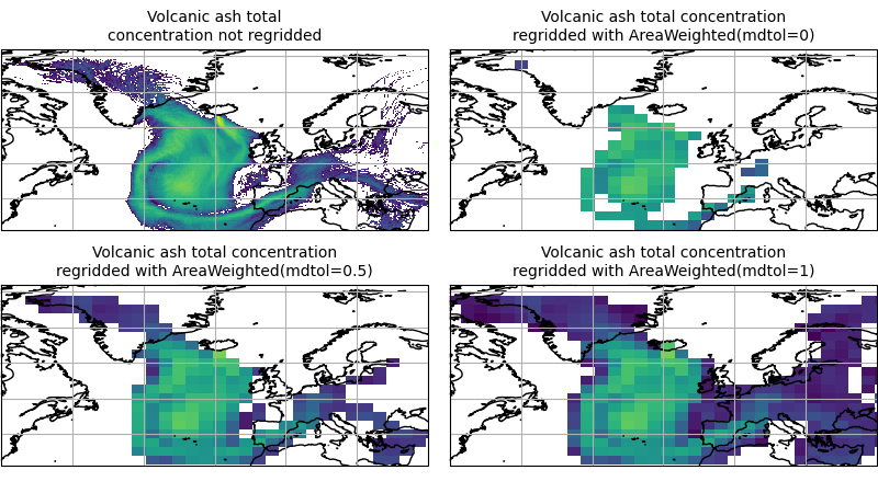
To visualise the above regrid, let’s plot the original data, along with 3 distinct
mdtol values to compare the result:
(Source code, png)
Caching a Regridder
If you need to regrid multiple cubes with a common source grid onto a common target grid you can ‘cache’ a regridder to be used for each of these regrids. This can shorten the execution time of your code as the most computationally intensive part of a regrid is setting up the regridder.
To cache a regridder you must set up a regridder scheme and call the scheme’s regridder method. The regridder method takes as arguments:
a cube (that is to be regridded) defining the source grid, and
a cube defining the target grid to regrid the source cube to.
For example:
>>> global_air_temp = iris.load_cube(iris.sample_data_path('air_temp.pp'))
>>> rotated_psl = iris.load_cube(iris.sample_data_path('rotated_pole.nc'))
>>> regridder = iris.analysis.Nearest().regridder(global_air_temp, rotated_psl)
When this cached regridder is called you must pass it a cube on the same grid
as the source grid cube (in this case global_air_temp) that is to be
regridded to the target grid. For example:
>>> for cube in list_of_cubes_on_source_grid:
...     result = regridder(cube)
In each case result will be the input cube regridded to the grid defined by
the target grid cube (in this case rotated_psl) that we used to define the
cached regridder.
Regridding Lazy Data
If you are working with large cubes, especially when you are regridding to a high resolution target grid, you may run out of memory when trying to regrid a cube. When this happens, make sure the input cube has lazy data
>>> air_temp = iris.load_cube(iris.sample_data_path('A1B_north_america.nc'))
>>> air_temp
<iris 'Cube' of air_temperature / (K) (time: 240; latitude: 37; longitude: 49)>
>>> air_temp.has_lazy_data()
True
and the regridding scheme supports lazy data. All regridding schemes described here support lazy data. If you still run out of memory even while using lazy data, inspect the chunks :
>>> air_temp.lazy_data().chunks
((240,), (37,), (49,))
The cube above consist of a single chunk, because it is fairly small. For larger cubes, iris will automatically create chunks of an optimal size when loading the data. However, because regridding to a high resolution grid may dramatically increase the size of the data, the automatically chosen chunks might be too large.
As an example of how to solve this, we could manually re-chunk the time dimension, to regrid it in 8 chunks of 30 timesteps at a time:
>>> air_temp.data = air_temp.lazy_data().rechunk([30, None, None])
>>> air_temp.lazy_data().chunks
((30, 30, 30, 30, 30, 30, 30, 30), (37,), (49,))
Assuming that Dask is configured such that it processes only a few chunks of the data array at a time, this will further reduce memory use.
Note that chunking in the horizontal dimensions is not supported by the regridding schemes. Chunks in these dimensions will automatically be combined before regridding.