Note
Click here to download the full example code
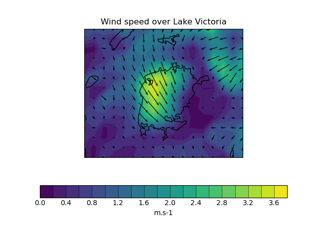
Plotting Wind Direction Using Quiver
This example demonstrates using quiver to plot wind speed contours and wind direction arrows from wind vector component input data. The vector components are co-located in space in this case.
For the second plot, the data used for the arrows is normalised to produce arrows with a uniform size on the plot.

import cartopy.feature as cfeat
import matplotlib.pyplot as plt

import iris
import iris.plot as iplt
import iris.quickplot as qplt


def main():
    # Load the u and v components of wind from a pp file.
    infile = iris.sample_data_path("wind_speed_lake_victoria.pp")

    uwind = iris.load_cube(infile, "x_wind")
    vwind = iris.load_cube(infile, "y_wind")

    # Create a cube containing the wind speed.
    windspeed = (uwind**2 + vwind**2) ** 0.5
    windspeed.rename("windspeed")

    # Plot the wind speed as a contour plot.
    qplt.contourf(windspeed, 20)

    # Show the lake on the current axes.
    lakes = cfeat.NaturalEarthFeature(
        "physical", "lakes", "50m", facecolor="none"
    )
    plt.gca().add_feature(lakes)

    # Add arrows to show the wind vectors.
    iplt.quiver(uwind, vwind, pivot="middle")

    plt.title("Wind speed over Lake Victoria")
    qplt.show()

    # Normalise the data for uniform arrow size.
    u_norm = uwind / windspeed
    v_norm = vwind / windspeed

    # Make a new figure for the normalised plot.
    plt.figure()

    qplt.contourf(windspeed, 20)
    plt.gca().add_feature(lakes)
    iplt.quiver(u_norm, v_norm, pivot="middle")

    plt.title("Wind speed over Lake Victoria")
    qplt.show()


if __name__ == "__main__":
    main()
Total running time of the script: ( 0 minutes 0.944 seconds)