2. Parallelising a Loop of Multiple Calls to a Third Party Library

Whilst Iris does provide extensive functionality for performing statistical and mathematical operations on your data, it is sometimes necessary to use a third party library.

The following example describes a real world use case of how to parallelise multiple calls to a third party library using dask bags.

2.1 The Problem - Parallelising a Loop

In this particular example, the user is calculating a sounding parcel for each column in their dataset. The cubes that are used are of shape:

(model_level_number: 20; grid_latitude: 1536; grid_longitude: 1536)

As a sounding is calculated for each column, this means there are 1536x1536 individual calculations.

In Python, it is common practice to vectorize the calculation of for loops. Vectorising is done by using NumPy to operate on the whole array at once rather than a single element at a time. Unfortunately, not all operations are vectorisable, including the calculation in this example, and so we look to other methods to improve the performance.

2.2 Original Code with Loop

We start out by loading cubes of pressure, temperature, dewpoint temperature and height:

import iris
import numpy as np
from skewt import SkewT as sk

pressure = iris.load_cube('a.press.19981109.pp')
temperature = iris.load_cube('a.temp.19981109.pp')
dewpoint = iris.load_cube('a.dewp.19981109.pp')
height = iris.load_cube('a.height.19981109.pp')

We set up the NumPy arrays we will be filling with the output data:

output_arrays = [np.zeros(pressure.shape[0]) for _ in range(6)]
cape, cin, lcl, lfc, el, tpw = output_data

Now we loop over the columns in the data to calculate the soundings:

for y in range(nlim):
    for x in range(nlim):
        mydata = {'pres': pressure[:, y, x],
                  'temp': temperature[:, y, x],
                  'dwpt': dewpoint[:, y, x],
                  'hght': height[:, y, x]}

        # Calculate the sounding with the selected column of data.
        S = sk.Sounding(soundingdata=mydata)
        try:
            startp, startt, startdp, type_ = S.get_parcel(parcel_def)
            P_lcl, P_lfc, P_el, CAPE, CIN = S.get_cape(
                startp, startt, startdp, totalcape='tot')
        TPW = S.precipitable_water()
        except:
            P_lcl, P_lfc, P_el, CAPE, CIN, TPW = [
                np.ma.masked for _ in range(6)]

        # Fill the output arrays with the results
        cape[y,x] = CAPE
        cin[y,x] = CIN
        lcl[y,x] = P_lcl
        lfc[y,x] = P_lfc
        el[y,x] = P_el
        tpw[y,x] = TPW

2.3 Profiling the Code with Kapture

Kapture is a useful statistical profiler. For more information see the Kapture repo.

Results below:

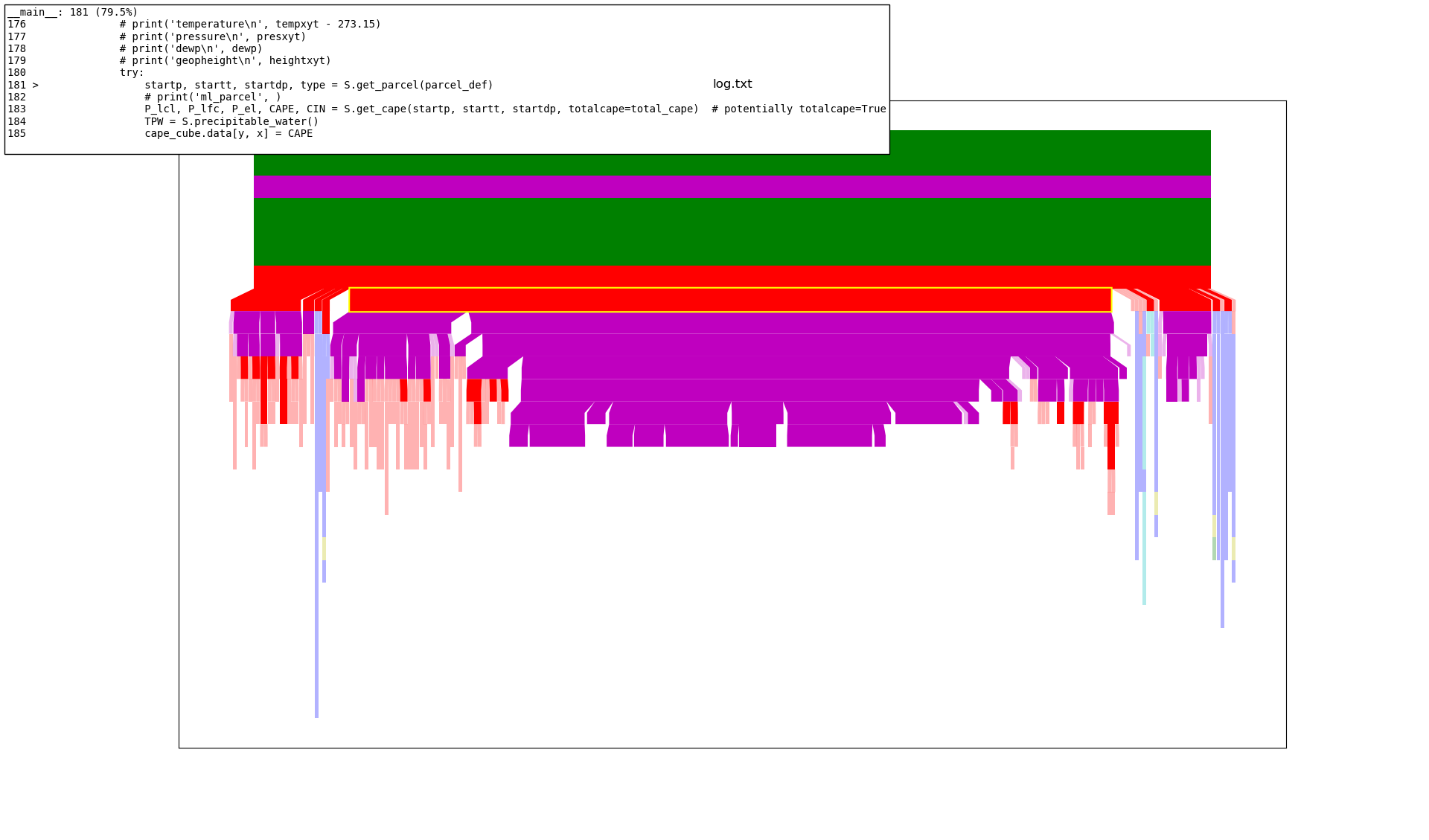
As we can see above, (looking at the highlighted section of the red bar) it spends most of the time in the call to

S.get_parcel(parcel_def)

As there are over two million columns in the data, we would greatly benefit from parallelising this work.

2.4 Parallelising with Dask Bags

Dask bags are collections of Python objects that you can map a computation over in a parallel manner.

For more information about dask bags, see the Dask Bag Documentation.

Dask bags work best with lightweight objects, so we will create a collection of indices into our data arrays.

First, we put the loop into a function that takes a slice object to index the appropriate section of the array.:

def calculate_sounding(y_slice):
    for y in range(y_slice.stop-y_slice.start):
        for x in range(nlim):
            mydata = {'pres': pressure[:, y_slice][:, y, x],
                      'temp': temperature[:, y_slice][:, y, x],
                      'dwpt': dewpoint[:, y_slice][:, y, x],
                      'hght': height[:, y_slice][:, y, x]}

            # Calculate the sounding with the selected column of data.
            S = sk.Sounding(soundingdata=mydata)
            try:
                startp, startt, startdp, type_ = S.get_parcel(parcel_def)
                P_lcl, P_lfc, P_el, CAPE, CIN = S.get_cape(
                    startp, startt, startdp, totalcape=total_cape)
                TPW = S.precipitable_water()
            except:
                P_lcl, P_lfc, P_el, CAPE, CIN, TPW = [
                    np.ma.masked for _ in range(6)]

            # Fill the output arrays with the results
            cape[:, y_slice][y,x] = CAPE
            cin[:, y_slice][y,x] = CIN
            lcl[:, y_slice][y,x] = P_lcl
            lfc[:, y_slice][y,x] = P_lfc
            el[:, y_slice][y,x] = P_el
            tpw[:, y_slice][y,x] = TPW

Then we create a dask bag of slice objects that will create multiple partitions along the y axis.:

num_of_workers = 4
len_of_y_axis = pressure.shape[1]

part_loc = [int(loc) for loc in np.floor(np.linspace(0, len_of_y_axis,
                                                     num_of_workers + 1))]

dask_bag = db.from_sequence(
    [slice(part_loc[i], part_loc[i+1]) for i in range(num_of_workers)])

with dask.config.set(scheduler='processes'):
    dask_bag.map(calculate_sounding).compute()

When this was run on a machine with 4 workers, a speedup of ~4x was achieved, as expected.

Note that if using the processes scheduler this is some extra time spent serialising the data to pass it between workers. For more information on the different schedulers available in Dask, see Dask Scheduler Overview.

For more speed up, it is possible to run the same code on a multi-processing system where you will have access to more CPUs.

In this particular example, we are handling multiple numpy arrays and so we use dask bags. If working with a single numpy array, it may be more appropriate to use Dask Arrays (see Dask Arrays for more information).

2.5 Lessons

• If possible, dask bags should contain lightweight objects

• Minimise the number of tasks that are created