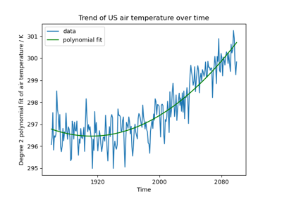
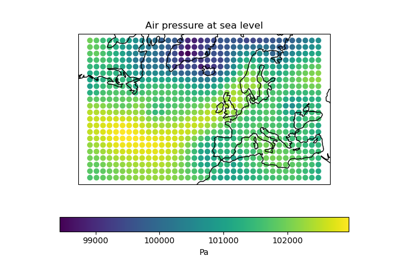
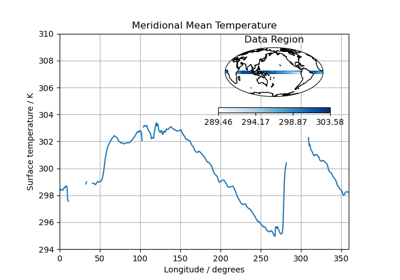
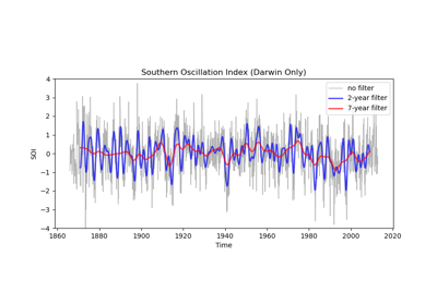
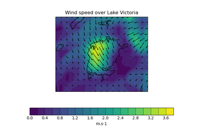
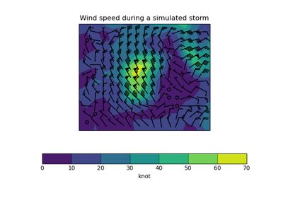
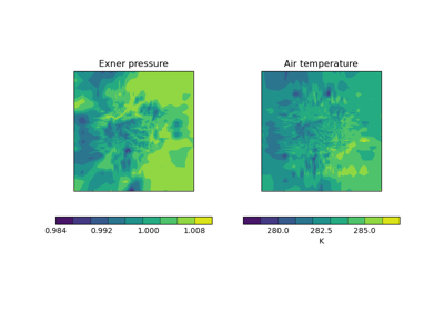
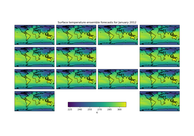
Logo
stable

Getting Started

  • Installing Iris
  • Gallery
    • General
      • Example of a Polar Stereographic Plot
      • Quickplot of a 2D Cube on a Map
      • Cross Section Plots
      • Multi-Line Temperature Profile Plot
      • Fitting a Polynomial
      • Rotated Pole Mapping
      • Test Data Showing Inset Plots
      • Applying a Filter to a Time-Series
      • Deriving the Coriolis Frequency Over the Globe
      • Calculating a Custom Statistic
      • Colouring Anomaly Data With Logarithmic Scaling
      • Plotting in Different Projections
      • Loading a Cube From a Custom File Format
    • Meteorology
      • Ionosphere Space Weather
      • Hovmoller Diagram of Monthly Surface Temperature
      • Plotting Wind Direction Using Quiver
      • Deriving Exner Pressure and Air Temperature
      • Global Average Annual Temperature Plot
      • Seasonal Ensemble Model Plots
      • Global Average Annual Temperature Maps
    • Oceanography
      • Tri-Polar Grid Projected Plotting
      • Load a Time Series of Data From the NEMO Model
      • Oceanographic Profiles and T-S Diagrams

User Guide

  • Introduction
  • Iris Data Structures
  • Loading Iris Cubes
  • Saving Iris Cubes
  • Navigating a Cube
  • Subsetting a Cube
  • Real and Lazy Data
  • Plotting a Cube
  • Cube Interpolation and Regridding
  • Merge and Concatenate
  • Cube Statistics
  • Cube Maths
  • Citing Iris
  • Code Maintenance

Further Topics

  • Introduction
  • Metadata
  • Lenient Metadata
  • Lenient Cube Maths

Developers Guide

  • Getting Involved
  • Working With Iris Source Code
  • Contributing to the Documentation
  • Contributing to the Code Base
  • Contributing Your Changes
  • Releases

Reference

  • Iris API
  • What’s New in Iris
  • Iris Technical Papers
  • Iris Copyright, Licensing and Contributors

Support

  • Source Code
  • Users Google Group
  • Developers Google Group
  • StackOverflow for "How Do I?"
  • Legacy Documentation
Iris
  • Docs »
  • Gallery
  • Edit on GitHub

Gallery

The gallery is divided into sections as described below. All entries show the code used to produce the example plot. Additionally there are links to download the code directly as source or as part of a jupyter notebook, these links are at the bottom of the page.

In order to successfully view the jupyter notebook locally so you may experiment with the code you will need an environment setup with the appropriate dependencies, see Installing Iris for instructions. Ensure that iris-sample-data is installed as it is used in the gallery. Additionally ensure that you install jupyter. The command to install both is:

conda install -c conda-forge iris-sample-data jupyter

Once you have downloaded the notebooks (bottom of each gallery page), you may start the jupyter notebook via:

jupyter notebook

If you wish to contribute to the gallery see the Gallery section of the Contributing to the Documentation.

General

Example of a Polar Stereographic Plot

Figure 1 Example of a Polar Stereographic Plot

Quickplot of a 2D Cube on a Map

Figure 2 Quickplot of a 2D Cube on a Map

Cross Section Plots

Figure 3 Cross Section Plots

Multi-Line Temperature Profile Plot

Figure 4 Multi-Line Temperature Profile Plot

Fitting a Polynomial

Figure 5 Fitting a Polynomial

Rotated Pole Mapping

Figure 6 Rotated Pole Mapping

Test Data Showing Inset Plots

Figure 7 Test Data Showing Inset Plots

Applying a Filter to a Time-Series

Figure 8 Applying a Filter to a Time-Series

Deriving the Coriolis Frequency Over the Globe

Figure 9 Deriving the Coriolis Frequency Over the Globe

Calculating a Custom Statistic

Figure 10 Calculating a Custom Statistic

Colouring Anomaly Data With Logarithmic Scaling

Figure 11 Colouring Anomaly Data With Logarithmic Scaling

Plotting in Different Projections

Figure 12 Plotting in Different Projections

Loading a Cube From a Custom File Format

Figure 13 Loading a Cube From a Custom File Format

Meteorology

Ionosphere Space Weather

Figure 14 Ionosphere Space Weather

Hovmoller Diagram of Monthly Surface Temperature

Figure 15 Hovmoller Diagram of Monthly Surface Temperature

Plotting Wind Direction Using Quiver

Figure 16 Plotting Wind Direction Using Quiver

Deriving Exner Pressure and Air Temperature

Figure 17 Deriving Exner Pressure and Air Temperature

Global Average Annual Temperature Plot

Figure 18 Global Average Annual Temperature Plot

Seasonal Ensemble Model Plots

Figure 19 Seasonal Ensemble Model Plots

Global Average Annual Temperature Maps

Figure 20 Global Average Annual Temperature Maps

Oceanography

Tri-Polar Grid Projected Plotting

Figure 21 Tri-Polar Grid Projected Plotting

Load a Time Series of Data From the NEMO Model

Figure 22 Load a Time Series of Data From the NEMO Model

Oceanographic Profiles and T-S Diagrams

Figure 23 Oceanographic Profiles and T-S Diagrams

Download all examples in Python source code: gallery_python.zip

Download all examples in Jupyter notebooks: gallery_jupyter.zip

Gallery generated by Sphinx-Gallery

Next Previous

© Copyright Iris Contributors Revision f468da3c.

Built with Sphinx using a theme provided by Read the Docs.
Read the Docs v: stable
Versions
latest
stable
v3.0.1
v3.0.x
v3.0.0
v3.0.0rc0
Downloads
pdf
html
On Read the Docs
Project Home
Builds

Free document hosting provided by Read the Docs.