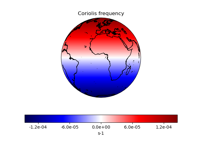
Deriving the Coriolis Frequency Over the Globe

This code computes the Coriolis frequency and stores it in a cube with associated metadata. It then plots the Coriolis frequency on an orthographic projection.

import cartopy.crs as ccrs
import matplotlib.pyplot as plt
import numpy as np

import iris
from iris.coord_systems import GeogCS
import iris.plot as iplt


def main():
    # Start with arrays for latitudes and longitudes, with a given number of
    # coordinates in the arrays.
    coordinate_points = 200
    longitudes = np.linspace(-180.0, 180.0, coordinate_points)
    latitudes = np.linspace(-90.0, 90.0, coordinate_points)
    lon2d, lat2d = np.meshgrid(longitudes, latitudes)

    # Omega is the Earth's rotation rate, expressed in radians per second
    omega = 7.29e-5

    # The data for our cube is the Coriolis frequency,
    # `f = 2 * omega * sin(phi)`, which is computed for each grid point over
    # the globe from the 2-dimensional latitude array.
    data = 2.0 * omega * np.sin(np.deg2rad(lat2d))

    # We now need to define a coordinate system for the plot.
    # Here we'll use GeogCS; 6371229 is the radius of the Earth in metres.
    cs = GeogCS(6371229)

    # The Iris coords module turns the latitude list into a coordinate array.
    # Coords then applies an appropriate standard name and unit to it.
    lat_coord = iris.coords.DimCoord(
        latitudes, standard_name="latitude", units="degrees", coord_system=cs
    )

    # The above process is repeated for the longitude coordinates.
    lon_coord = iris.coords.DimCoord(
        longitudes, standard_name="longitude", units="degrees", coord_system=cs
    )

    # Now we add bounds to our latitude and longitude coordinates.
    # We want simple, contiguous bounds for our regularly-spaced coordinate
    # points so we use the guess_bounds() method of the coordinate. For more
    # complex coordinates, we could derive and set the bounds manually.
    lat_coord.guess_bounds()
    lon_coord.guess_bounds()

    # Now we input our data array into the cube.
    new_cube = iris.cube.Cube(
        data,
        standard_name="coriolis_parameter",
        units="s-1",
        dim_coords_and_dims=[(lat_coord, 0), (lon_coord, 1)],
    )

    # Now let's plot our cube, along with coastlines, a title and an
    # appropriately-labelled colour bar:
    ax = plt.axes(projection=ccrs.Orthographic())
    ax.coastlines(resolution="10m")
    mesh = iplt.pcolormesh(new_cube, cmap="seismic")
    tick_levels = [-0.00012, -0.00006, 0.0, 0.00006, 0.00012]
    plt.colorbar(
        mesh,
        orientation="horizontal",
        label="s-1",
        ticks=tick_levels,
        format="%.1e",
    )
    plt.title("Coriolis frequency")
    plt.show()


if __name__ == "__main__":
    main()