Load a Time Series of Data From the NEMO Model

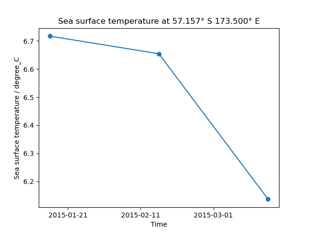
This example demonstrates how to load multiple files containing data output by the NEMO model and combine them into a time series in a single cube. The different time dimensions in these files can prevent Iris from concatenating them without the intervention shown here.

import matplotlib.pyplot as plt

import iris
import iris.plot as iplt
import iris.quickplot as qplt
from iris.util import equalise_attributes, promote_aux_coord_to_dim_coord


def main():
    # Load the three files of sample NEMO data.
    fname = iris.sample_data_path("NEMO/nemo_1m_*.nc")
    cubes = iris.load(fname)

    # Some attributes are unique to each file and must be removed to allow
    # concatenation.
    equalise_attributes(cubes)

    # The cubes still cannot be concatenated because their dimension coordinate
    # is "time_counter", which has the same value for each cube.  concatenate
    # needs distinct values in order to create a new DimCoord for the output
    # cube.  Here, each cube has a "time" auxiliary coordinate, and these do
    # have distinct values, so we can promote them to allow concatenation.
    for cube in cubes:
        promote_aux_coord_to_dim_coord(cube, "time")

    # The cubes can now be concatenated into a single time series.
    cube = cubes.concatenate_cube()

    # Generate a time series plot of a single point
    plt.figure()
    y_point_index = 100
    x_point_index = 100
    qplt.plot(cube[:, y_point_index, x_point_index], "o-")

    # Include the point's position in the plot's title
    lat_point = cube.coord("latitude").points[y_point_index, x_point_index]
    lat_string = "{:.3f}\u00b0 {}".format(
        abs(lat_point), "N" if lat_point > 0.0 else "S"
    )
    lon_point = cube.coord("longitude").points[y_point_index, x_point_index]
    lon_string = "{:.3f}\u00b0 {}".format(
        abs(lon_point), "E" if lon_point > 0.0 else "W"
    )
    plt.title("{} at {} {}".format(cube.long_name.capitalize(), lat_string, lon_string))

    iplt.show()


if __name__ == "__main__":
    main()