Note
Go to the end to download the full example code.
Plotting Wind Direction Using Quiver#
How to use Iris to plot wind quivers. |
Tags: topic_plotting
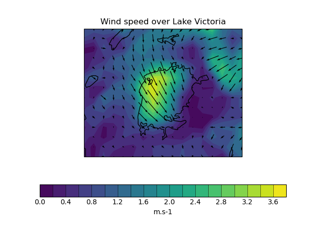
This example demonstrates using quiver to plot wind speed contours and wind direction arrows from wind vector component input data. The vector components are co-located in space in this case.
For the second plot, the data used for the arrows is normalised to produce arrows with a uniform size on the plot.

import cartopy.feature as cfeat
import matplotlib.pyplot as plt

import iris
import iris.plot as iplt
import iris.quickplot as qplt


def main():
    # Load the u and v components of wind from a pp file.
    infile = iris.sample_data_path("wind_speed_lake_victoria.pp")

    uwind = iris.load_cube(infile, "x_wind")
    vwind = iris.load_cube(infile, "y_wind")

    # Create a cube containing the wind speed.
    windspeed = (uwind**2 + vwind**2) ** 0.5
    windspeed.rename("windspeed")

    # Plot the wind speed as a contour plot.
    qplt.contourf(windspeed, 20)

    # Show the lake on the current axes.
    lakes = cfeat.NaturalEarthFeature("physical", "lakes", "50m", facecolor="none")
    plt.gca().add_feature(lakes)

    # Add arrows to show the wind vectors.
    iplt.quiver(uwind, vwind, pivot="middle")

    plt.title("Wind speed over Lake Victoria")
    qplt.show()

    # Normalise the data for uniform arrow size.
    u_norm = uwind / windspeed
    v_norm = vwind / windspeed

    # Make a new figure for the normalised plot.
    plt.figure()

    qplt.contourf(windspeed, 20)
    plt.gca().add_feature(lakes)
    iplt.quiver(u_norm, v_norm, pivot="middle")

    plt.title("Wind speed over Lake Victoria")
    qplt.show()


if __name__ == "__main__":
    main()
Total running time of the script: (0 minutes 0.543 seconds)