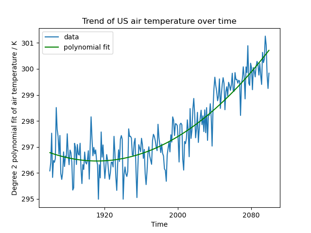
Fitting a Polynomial

This example demonstrates computing a polynomial fit to 1D data from an Iris cube, adding the fit to the cube’s metadata, and plotting both the 1D data and the fit.

import matplotlib.pyplot as plt
import numpy as np

import iris
import iris.quickplot as qplt


def main():
    # Load some test data.
    fname = iris.sample_data_path("A1B_north_america.nc")
    cube = iris.load_cube(fname)

    # Extract a single time series at a latitude and longitude point.
    location = next(cube.slices(["time"]))

    # Calculate a polynomial fit to the data at this time series.
    x_points = location.coord("time").points
    y_points = location.data
    degree = 2

    p = np.polyfit(x_points, y_points, degree)
    y_fitted = np.polyval(p, x_points)

    # Add the polynomial fit values to the time series to take
    # full advantage of Iris plotting functionality.
    long_name = "degree_{}_polynomial_fit_of_{}".format(degree, cube.name())
    fit = iris.coords.AuxCoord(y_fitted, long_name=long_name, units=location.units)
    location.add_aux_coord(fit, 0)

    qplt.plot(location.coord("time"), location, label="data")
    qplt.plot(
        location.coord("time"),
        location.coord(long_name),
        "g-",
        label="polynomial fit",
    )
    plt.legend(loc="best")
    plt.title("Trend of US air temperature over time")

    qplt.show()


if __name__ == "__main__":
    main()