Patterns for working with temporal coordinates.

Tags: topic_data_model | topic_plotting

Temporal Coordinates#

Here we provide some handy patterns and tips for working with temporal coordinates i.e., time coordinates.

Introduction#

First, let’s familiarise ourselves with the time coordinate that we’ll be working with:

>>> tcoord = cube.coord("time")
>>> tcoord
<DimCoord: time / (hours since 1970-01-01 00:00:00)  [...]  shape(6,)>

Let’s break down this coordinate summary so that we understand each of its individual components:

DimCoord - This is the coordinate type, which may be either a DimCoord or AuxCoord. A dimensional coordinate (DimCoord) must be numeric, strictly monotonic, have no missing data, and at most 1D. Otherwise, it’s an auxiliary coordinate (AuxCoord), which is not restricted by data type nor dimensionality.
time - This is the name of the coordinate. The name is derived firstly from the coordinate standard_name. Failing that, the long_name is used, otherwise the var_name before defaulting to a value of unknown.
hours since 1970-01-01 00:00:00 - This tells us the coordinates temporal units of measure (hours) relative to its epoch (1970-01-01 00:00:00).
[...] - Represents the temporal points, the values of which are not displayed in this shortend summary. However, note that if the coordinate had bounds this would be represented as [...]+bounds.
shape(6,) - Tells us that the coordinate has one dimension containing 6 points.

We can easily inspect the points contained within our tcoord:

>>> tcoord.points
array([347926.16666667, 347926.33333333, 347926.5       , 347926.66666667,
   347926.83333333, 347927.        ])

However, these raw values are pretty meaningless on their own. As hinted to above, these points are measured in units of hours relative to the epoch 1970-01-01 00:00:00. The metadata defining all this information is available from the units attribute of the coordinate:

>>> tcoord.units
Unit('hours since 1970-01-01 00:00:00', calendar='standard')

Note

All temporal coordinates have a calendar attribute associated with their units.

In this case our tcoord has a standard (or gregorian) calendar and we can convert its hard to understand raw values into meaningful date/time (YYYY-MM-DD HH:MM:SS) representations relative to its calendar and epoch:

>>> print(tcoord)
DimCoord :  time / (hours since 1970-01-01 00:00:00, standard calendar)
points: [
    2009-09-09 22:10:00, 2009-09-09 22:20:00, 2009-09-09 22:30:00,
    2009-09-09 22:40:00, 2009-09-09 22:50:00, 2009-09-09 23:00:00]
shape: (6,)
dtype: float64
standard_name: 'time'

Now we can clearly see that our tcoord time interval commences on 2009-09-09 at 22:10:00 with samples that are each 10 minutes apart.

Note that our tcoord does not have any bounds associated with it:

>>> tcoord.has_bounds()
False
>>> tcoord.bounds is None
True

However, as a convenience, we can guess the bounds of a coordinate using its guess_bounds() method:

>>> tcoord.guess_bounds()
>>> print(tcoord)
DimCoord :  time / (hours since 1970-01-01 00:00:00, standard calendar)
points: [
    2009-09-09 22:10:00, 2009-09-09 22:20:00, 2009-09-09 22:30:00,
    2009-09-09 22:40:00, 2009-09-09 22:50:00, 2009-09-09 23:00:00]
bounds: [
    [2009-09-09 22:05:00, 2009-09-09 22:15:00],
    [2009-09-09 22:15:00, 2009-09-09 22:25:00],
    [2009-09-09 22:25:00, 2009-09-09 22:35:00],
    [2009-09-09 22:35:00, 2009-09-09 22:45:00],
    [2009-09-09 22:45:00, 2009-09-09 22:55:00],
    [2009-09-09 22:55:00, 2009-09-09 23:05:00]]
shape: (6,)  bounds(6, 2)
dtype: float64
standard_name: 'time'

Warning

guess_bounds() is an in-place operation.

Indexing#

Coordinates are first-class-citizens and may be indexed akin to other python built-in types such as lists or tuples.

As an example, let’s index the last sample of the tcoord:

>>> tsample = tcoord[-1]
>>> print(tsample)
DimCoord :  time / (hours since 1970-01-01 00:00:00, standard calendar)
points: [2009-09-09 23:00:00]
bounds: [[2009-09-09 22:55:00, 2009-09-09 23:05:00]]
shape: (1,)  bounds(1, 2)
dtype: float64
standard_name: 'time'

Note

Indexing a coordinate returns a new instance of the same coordinate type i.e., AuxCoord or DimCoord, populated with all the metadata and associated data i.e., points, or points and bounds, at the given index/indices.

In the above example, indexing the tcoord yields a scalar DimCoord which we can sanity check for equivalence:

>>> tsample == tcoord[-1]
True

A lighter-weight indexing solution is to leverage the cell() method instead:

>> tcell = tcoord.cell(-1)
>> tcell
Cell(point=cftime.DatetimeGregorian(2009, 9, 9, 23, 0, 0, 0, has_year_zero=False), bound=(cftime.DatetimeGregorian(2009, 9, 9, 22, 55, 0, 0, has_year_zero=False), cftime.DatetimeGregorian(2009, 9, 9, 23, 5, 0, 0, has_year_zero=False)))

This returns a Cell object rather than a coordinate, which only contains the point, or point and bound at the given index:

>>> tcell.point
cftime.DatetimeGregorian(2009, 9, 9, 23, 0, 0, 0, has_year_zero=False)
>>> tcell.bound
(cftime.DatetimeGregorian(2009, 9, 9, 22, 55, 0, 0, has_year_zero=False), cftime.DatetimeGregorian(2009, 9, 9, 23, 5, 0, 0, has_year_zero=False))

Warning

A temporal Cell will always contain cftime objects rather than native python datetime objects.

The tsample (DimCoord) and tcell (Cell) were both generated from the same index of tcoord. However, the tsample does not contain rich date/time objects, rather it contains numerical offsets measured relative to the calendar and epoch defined within its units:

>>> tsample.units
Unit('hours since 1970-01-01 00:00:00', calendar='standard')
>>> tsample.points
array([347927.])
>>> tsample.bounds
array([[347926.91666667, 347927.08333333]])

To convert these points and bounds into equivalent tcell cftime objects, apply the following pattern:

>>> tsample.units.num2date(tsample.points)
array([cftime.DatetimeGregorian(2009, 9, 9, 23, 0, 0, 0, has_year_zero=False)],
  dtype=object)
>>> tsample.units.num2date(tsample.bounds)
array([[cftime.DatetimeGregorian(2009, 9, 9, 22, 55, 0, 0, has_year_zero=False),
    cftime.DatetimeGregorian(2009, 9, 9, 23, 5, 0, 0, has_year_zero=False)]],
  dtype=object)

Iteration#

Akin to indexing, we can also iterate over coordinates just as you would naturally with other python built-in types such as lists or tuples.

For example, given our tcoord:

>>> print(tcoord)
DimCoord :  time / (hours since 1970-01-01 00:00:00, standard calendar)
points: [
    2009-09-09 22:10:00, 2009-09-09 22:20:00, 2009-09-09 22:30:00,
    2009-09-09 22:40:00, 2009-09-09 22:50:00, 2009-09-09 23:00:00]
bounds: [
    [2009-09-09 22:05:00, 2009-09-09 22:15:00],
    [2009-09-09 22:15:00, 2009-09-09 22:25:00],
    [2009-09-09 22:25:00, 2009-09-09 22:35:00],
    [2009-09-09 22:35:00, 2009-09-09 22:45:00],
    [2009-09-09 22:45:00, 2009-09-09 22:55:00],
    [2009-09-09 22:55:00, 2009-09-09 23:05:00]]
shape: (6,)  bounds(6, 2)
dtype: float64
standard_name: 'time'

We can easily iterate over each index:

>>> from pprint import pprint
>>> pprint(list(tcoord))
[<DimCoord: time / (hours since 1970-01-01 00:00:00)  [2009-09-09 22:10:00]+bounds>,
 <DimCoord: time / (hours since 1970-01-01 00:00:00)  [2009-09-09 22:20:00]+bounds>,
 <DimCoord: time / (hours since 1970-01-01 00:00:00)  [2009-09-09 22:30:00]+bounds>,
 <DimCoord: time / (hours since 1970-01-01 00:00:00)  [2009-09-09 22:40:00]+bounds>,
 <DimCoord: time / (hours since 1970-01-01 00:00:00)  [2009-09-09 22:50:00]+bounds>,
 <DimCoord: time / (hours since 1970-01-01 00:00:00)  [2009-09-09 23:00:00]+bounds>]

Note that this is functionally equivalent to the following:

pprint([sample for sample in tcoord])

Both of the above patterns generate a list of scalar DimCoord objects at each coordinate index in tcoord.

Note

Iterating over a coordinate returns a new instance of the same coordinate type i.e., AuxCoord or DimCoord, populated with all the metadata and associated data i.e., points, or points and bounds, for each coordinate index.

Alternatively, we can use the cells() method to generate lighter-weight Cell objects for each coordinate index rather than DimCoord objects.

`cftime` vs `datetime`#

Depending on your workflow, you may wish to deal directly with either cftime objects or native python datetime objects rather than raw temporal values within the points/bounds of a coordinate.

There are several different ways to convert raw temporal values, so let’s consolidating our understanding and enumerate the various options available to us.

`cftime`#

The direct approach is to leverage either of the cell() or cells() methods. Both of which provide one or more Cell objects.

A temporal Cell will always contain cftime objects for its point, or point and bound.

`datetime`#

Converting raw temporal values to native python datetime objects is only valid for standard, gregorian or proleptic_gregorian calendar encoded data.

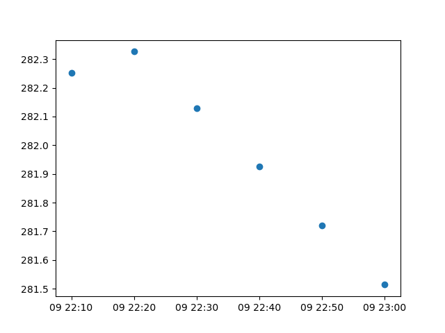
Plotting#

Creating a time-series plot is trivial when using iris.plot or iris.quickplot as they both handle cftime objects and native python datetime objects automatically.

For example:

Example 1 Plotting with iris#

import matplotlib.pyplot as plt

import iris
import iris.plot as iplt

fname = iris.sample_data_path("colpex.pp")
cube = iris.load_cube(fname, "air_potential_temperature")
tcoord = cube.coord("time")

iplt.scatter(tcoord, cube[:, 0, 0, 0])
plt.show()

Time-series scatter plot using iris.plot.scatter

Warning

Native matplotlib only supports python datetime objects.

Note that, iris.plot and iris.quickplot provide the convenience of also understanding iris objects, such as coordinates and cubes. However they also use the nc-time-axis package, which provides support for a cftime axis in matplotlib.

For comparison purposes, we can generate the same time-series scatter plot, but use nc-time-axis directly as follows:

Example 2 Plotting with nc-time-axis#

import matplotlib.pyplot as plt

import iris
import nc_time_axis

fname = iris.sample_data_path("colpex.pp")
cube = iris.load_cube(fname, "air_potential_temperature")
tcoord = cube.coord("time")

dates = tcoord.units.num2date(tcoord.points)
data = cube[:, 0, 0, 0].data

plt.scatter(dates, data)
plt.show()

Alternatively, we can manually convert our time-series values directly to datetime objects:

Example 3 Plotting with native datetime objects#

import matplotlib.pyplot as plt

import iris

fname = iris.sample_data_path("colpex.pp")
cube = iris.load_cube(fname, "air_potential_temperature")
tcoord = cube.coord("time")

dates = tcoord.units.num2pydate(tcoord.points)
data = cube[:, 0, 0, 0].data

plt.scatter(dates, data)
plt.show()

Temporal Coordinates#

Introduction#

Indexing#

Iteration#

cftime vs datetime#

cftime#

datetime#

Plotting#

`cftime` vs `datetime`#

`cftime`#

`datetime`#